Showing posts sorted by relevance for query LINE FOLLOWING. Sort by date Show all posts

line following robot proposal


Searches related to proposal line following robot

instructables line following robot
line following robot wikipedia
line following robot nxt
automated line following robot
sandwich line following robot
line following robot youtube
line following robot without microcontroller
line following robot pdf


line following robot proposal


Abstract

The line following is a classic introductory robot design and requires minimal amount of resources. This robot uses Microcontroller control. This robot is intended to showcase basic sensor design and robot control system in the form of a small autonomous robot which can follow a black line over white surface.

            A proposal for a line following robots and their relevance to engineering and society is given.  A project design for a line following robot is presented and discussed.  The project description is given, as well as the project approach, experiments to be run, and a proposed schedule for completing the robot.

The vehicle is supposed to have a low-resolution sensors and actuator. The control requirement, however, is specified so as to keep the vehicle as close as possible to the center of the line. The controllability issues are investigated, A multiple IR sensor based control algorithm is investigated for straight as well as curved paths. Experimental result is shown to demonstrate the usefulness of our idea. .


Final report using iandroid,line following robot 

line following,code in assembly language ,89s59,89s52 

Line following robot code in Arduino

Some Importantant links below with reports.just view the lik below
Arduino interesting projects:   
Arduino 30 simple and good projects 
Atmega projects lists
Android Electronics projects lists
Rf based Projects with report
engineering study notes 
GSM GPS based projects with report
Bluetooth based projects with reports


/* Robot Line Follow

/*wall tracking also same
 
 This sketch demonstrates the line following capabilities
 of the Arduino Robot. On the floor, place some black
 electrical tape along the path you wish the robot to follow.
 To indicate a stopping point, place another piece of tape
 perpendicular to the path.

 Circuit:
 * Arduino Robot

 created 1 May 2013
 by X. Yang
 modified 12 May 2013
 by D. Cuartielles

 This example is in the public domain
 */


#include <ArduinoRobot.h> // include the robot library

long timerOrigin; // used for counting elapsed time

void setup() {
  // initialize the Robot, SD card, display, and speaker
  Robot.begin();
  Robot.beginTFT();
  Robot.beginSD();
  Robot.beginSpeaker();

  // show the logots on the TFT screen
  Robot.displayLogos();
 
  Robot.drawBMP("lf.bmp", 0, 0); // display background image

  Robot.playFile("chase.sqm");  // play a song from the SD card
 
  // add the instructions
  Robot.text("Line Following\n\n place the robot on\n the track and \n see it run", 5, 5);
  Robot.text("Press the middle\n button to start...", 5, 61);
  Robot.waitContinue();

  // These are some general values that work for line following
  // uncomment one or the other to see the different behaviors of the robot
  // Robot.lineFollowConfig(11, 5, 50, 10);
  Robot.lineFollowConfig(11, 7, 60, 5);
 
  //set the motor board into line-follow mode
  Robot.setMode(MODE_LINE_FOLLOW);
 
  // start
  Robot.fill(255, 255, 255);
  Robot.stroke(255, 255, 255);
  Robot.rect(0, 0, 128, 80); // erase the previous text
  Robot.stroke(0, 0, 0);
  Robot.text("Start", 5, 5);
 
  Robot.stroke(0, 0, 0); // choose color for the text
  Robot.text("Time passed:", 5, 21); // write some text to the screen
 
  timerOrigin=millis(); // keep track of the elapsed time
 
  while(!Robot.isActionDone()) {  //wait for the finish signal
    Robot.debugPrint(millis()-timerOrigin, 5, 29);  // show how much time has passed
  }
 
  Robot.stroke(0, 0, 0);
  Robot.text("Done!", 5, 45);
}
void loop() {
  //nothing here, the program only runs once. Reset the robot
  //to do it again!
}

Some Importantant links below with reports.just view the lik below
Arduino interesting projects:   
Arduino 30 simple and good projects 
Atmega projects lists
Android Electronics projects lists
Rf based Projects with report
engineering study notes 
GSM GPS based projects with report
Bluetooth based projects with reports

Sample Electronics project proposal


1. Introduction


Fig (i) Block diagram of line following robot


2) Objective


3) Scope


4) Application.


5) Literature review


6) SOFTWARE AND HARDWARE


Expected result:-


7) Gantt chart


Conclusion
Bibliography


1)      Programming and Customizing the PIC microcontroller by Myke Predko
            PICmicro Mid-Range MCU Family Reference Manual by MICROCHIP
2)      PIC Robotics, A beginner’s guide to robotics projects using the PICmicro by John Malvirine  
3)      Plermjani inchuay, line follower robot: http://chaokhun.kmitl.ac.th/~kswichit/LFrobot/LFrobot.htm
4)      MUKUND22R, automated line following robot: http://letsmakerobots.com/node/31206


Line Follower Robot using Arduino


A line follower robot using 8051 microcontroller is already published here and this time the same thing is done using  arduino. This line follower robot is basically designed to follow a black line on a white surface. Any way the same project can be used to follow the opposite configuration with appropriate changes in the software. The entire hardware of this simple line follower robot using arduino can be divided into three parts. The sensor, arduino board and the motor driver circuit. Lets have a look at the sensor first.

Sensor.

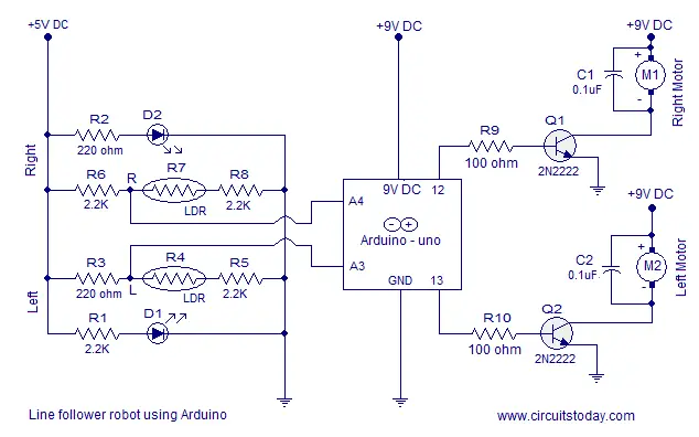
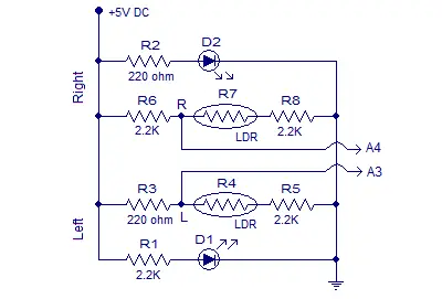
The sensor consists of two LED/LDR pairs with appropriate current limiting resistors. The resistance of an LDR is inversely proportional to the intensity of the light falling on it.  The circuit diagram of the sensor is shown in the figure below.
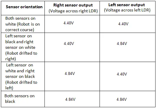
arduino line followerResistors R1 and R2 limits the current through the LEDs. Resistors R6, R8, R3,and R5 forms individual voltage divider networks in conjunction with the corresponding LDRs. When the sensor is correctly aligned, both LED/LDR pairs will over the white surface. In this condition sufficient amount of light gets reflected back to the LDRs and so their resistance will be low. So the voltage dropped across the LDR will be low. When the robot is drifted to  one side , the sensor in the opposite side falls over the black line and the intensity of light reflected back to the corresponding LDR  will be low. As a result the resistance of the LDR shoots up and the voltage dropped across it will be high. The voltages dropped across the right and left LDRs (nodes marked R and L in the above circuit)  are given as input to the analog input pins A4 and A3 of the Arduino board. Right and left sensor outputs observed while testing the above circuit is shown in the table below.
line follower robot using arduino

Arduino uno board.

The arduino board has to be programmed to keep the robot in correct path. This is done by reading the left and right sensor outputs and switching the left and right motors appropriately. Output of the right sensor is connected to the analog input A4 of the arduino and output of the left sensor is connected to the analog input A3 of the arduino. The voltage range that can be applied to a particular analog input of the arduino is 0 to 5V. This range can be converted into a digital value between 0 and 1023 using  analogRead () command.  For example if 3V is applied to A3,  the following code will return 3/(5/1023) which is equal to 613 in the variable leftValue.
int leftInput = A3;
int leftValue=0;
void loop ()
{
leftValue = analogRead (leftInput);
{
From the above table you can see that the voltage across a particular LDR will be 4.4V when it on white and 4.84V when it is on black. The digital equivalent of 4.4V will be 900 and that of 4.84V will be 990 as per the above scheme.  The median of these two values is 945 and it is set as the reference point for the program to check the orientation of the sensor module.
The program identifies the position of the sensor module by comparing the sensor readings with the reference point that is 945. If the reading of a particular sensor is greater than 945 the program can assume that the particular sensor is above black. If the reading of a particular sensor is less than 945 then it is assumed that the particular sensor is above white. If both sensor readings are less than 945 then it means both sensors are on white. If both sensor readings are above 945 it is assumed that both sensors are above black (the same thing happens if we lift the robot off the track). Based on the above four conditions, the program appropriately switches the left and right motors to keep the robot following the black line.

Motor driver.

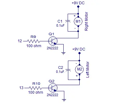
The motor driver circuit is based on two NPN transistors Q1 and Q2. Each transistors are wired as a switch with a resistor at its base for limiting the base current. The motors are connected to the emitter terminal of the corresponding transistors. A 0.1uF capacitor is connected across each motor  for by-passing the voltage spikes. Back emf  and arcing of brushes are the main reason behind the voltage spikes. If these voltage spikes are not by-passed it may affect the Arduino side.   Circuit diagram of the motor driver is shown in the figure below.
arduino line follower motor driver

Circuit diagram.

Full circuit diagram of the line follower robot  is shown in the figure below.
arduino line follower

Program.

int leftInput=A3;
int rightInput=A4;
int leftMotor=13;
int rightMotor=12;
int leftValue = 0;
int rightValue = 0;
void setup()
{
  pinMode (leftMotor, OUTPUT);
  pinMode (rightMotor, OUTPUT);
}
void loop()
{
  leftValue = analogRead (leftInput);
  rightValue= analogRead (rightInput);

 if
   ( leftValue < 945 && rightValue < 945)
   {
     digitalWrite (leftMotor, HIGH);
     digitalWrite (rightMotor, HIGH);
   }
   else
   {

     if
     ( leftValue > 945 && rightValue < 945)
    {
      digitalWrite (leftMotor, LOW);
      digitalWrite (rightMotor, HIGH);
    }
 else {
   if (leftValue < 945 && rightValue > 945)
   {
   digitalWrite (rightMotor, LOW);
   digitalWrite (leftMotor, HIGH);
   }
   else
   {
     if (leftValue > 945 && rightValue > 945)
     {digitalWrite (rightMotor, LOW);
       digitalWrite (leftMotor, LOW);
     }}
      }
    }}

Setting up the circuit.

  • First of all remember that each LED and LDR has its own characteristics.
  • Carefully measure the voltage across each LDRs in both scenarios (on white surface and black).
  • A lot of parameters like individual LDR/LED characteristics, ambient light, clearance between sensor and surface etc may affect the result.
  • Get in to your own reference point for the program. In my case it was 945 but you may get a different value.
  • Use a separate power supply unit for powering the motors. Anything above 100mA will be hard for the USB port.
  • The motors used here are 6V/30RPM DC bow motors. If such a configuration is not available, choose the closest one.
  • While soldering up the sensor module, the gap between the two LED/LDR pairs must be selected according to the width of the black line. In my case it was 2cm.
  • Clearance of the sensor from the ground was around 1cm in my case.
  • The sensor LEDs used were 4mm bright green LEDs.
  • The sensor LDRs used were general purpose LDRs.

line following robot code for atmega32

 line following robot code for atmega32


#ifndef F_CPU #define F_CPU 16000000UL // defines CPU frequency for delay frequency

  #endif

 #include <avr/io.h> // includes input/output header file

  #include <util/delay.h> // includes delay header file /*CODE FOR LINE FOLLOWER BY ROBOVITICS USING ATMEGA8 MICROCONTROLLER*/

  //******************************************************************** /* Connection of L293D IC with aTmega8. Pin2 (A1) of L293D is connected with PB2 (Pin 16 of aTmega8). Pin 7(B1) of L293D is connected with PB3 (MOSI) (PIN 17 of aTmega8) **A1 and B1 are the input pins of left side H-Bridge of L293D which is driving the left motor. Pin15 (A2) of L293D is connected with PB0 (Pin 14 of aTmega). Pin10 (B2) of L293D is connected with PB1(Pin15 of aTmega). Pin1 (EN1) and pin9 (EN2) is connected via motor enable switch. Pin3 and pin6 of L293D is connected with Left Motor. Pin14 and Pin11 of L293D is connected with right motor. */ // connect the left sensors on PC4 and right ones on PC5 

 int main(void)

 { DDRB=0b11111111;   //PORTB as output Port connected to motors

  DDRC=0b0000000;   //PORTC Input port connected to Sensors 

 int left_sensor=0, right_sensor=0; while(1)    // infinite loop

  {     

 left_sensor=PINC&0b0010000;      // mask PC4 bit of Port C 

 right_sensor=PINC&0b0100000;  // mask PC5 bit of Port C    

   if((left_sensor==0b0000000) & (right_sensor==0b0000000))  

    {               

   PORTB=0b00000000;   // stop       

  }  

 if((left_sensor==0b0010000) & (right_sensor==0b0100000))  

 {               

   PORTB=0b00001001;   // move straight      

         }

 if((left_sensor==0b0000000) & (right_sensor==0b0100000))          

     {              

    PORTB=0b00000001;   // turn left      

  } 

 if((left_sensor==0b0010000) & (right_sensor==0b0000000))         

      {                  PORTB=0b00001000;  // turn right        }   }   } 

*THE TEXT IN BLUE ARE THE COMMAND LINES


 over_turn(){PORTD&=0xF0;PORTD|=0x06; _delay_ms(900);right(); // over turn and changes direction _delay_ms(100);while(S4==0);stop();if(bot_dir==N){ bot_dir=S; return;}if(bot_dir==E){ bot_dir=W; return;}if(bot_dir==S){ bot_dir=N; return;}if(bot_dir==W){ bot_dir=E; return;}}reach_home() // function to take robot to initial cooridnate{ // many more condition exits according to robots direction of approching block, writethem if you want!step();

bot_y--;if(bot_x!=0){ left_ninety();while(bot_x)step();}if(bot_x==0){ if( bot_dir==N){ over_turn();while(bot_y)step();return;}if ( bot_dir==W){ left_ninety();while(bot_y)step();return;}}}void main (void){DDRB=0x00; // making PORTB as input

DDRA=0x00; // making PORTA as inputDDRD=0xFF; // making PORTD as outputPORTD=0x30; // setting Logic high on Enable pin of L293Dgrid_x=3; // setting maximun X coordinate of gridgrid_y=3; // setting maximum Y coordinate of gridbot_dir=1; // Initial robot direction , 1= North _delay_ms(1000); // a small delay before code startssearch(); // function to search for robotover_turn(); // make over turnreach_home(); // return to initial coordinate// line_follow();while(1); // stuck in a infinite loop after task is completed}

[Data Processing] An android based monitoring and alarm system for patients with chronic obtrusive disease.


Chapter 4

Data Processing

Following set up of the developed system, we proceed with the analysis, applied
for collected measurements: (1) change point detection, (2) anomaly detection,
(3) activity correlation. Each item is responsible for particular function and
represents different level of analysis. The first technique detects and registers
every unexpected sudden drop/jump during the monitoring process. The next
method, anomaly detection is aiming on detecting and highlighting unusual patterns
in the signal that might represent extra interest for a medical specialist.
Both algorithms are complementary and serve as a pre-step towards the on-line
monitoring system. Ideally, after change point is detected we should add other
parameters and perform correlation analysis. As it was discussed in Chapter 2
fuzzy logic can be used in this case to combine medical parameters and perform
a certain level of reasoning about patients health conditions. However, as
it was previously mentioned, particular qualities of the correlation are not thoroughly
verified when it comes to continuous datasets. Therefore it is essential
to conduct a series of experiments involving patients from different age groups
and with various diagnosis. After collecting this data we can apply the above
mentioned techniques to examine the nature of the correlation between medical
parameters involved in the monitoring. This will help to enhance the final
reasoning algorithm and avoid triggering an alarm when it is not necessary. Finally,
as a separate part of the correlation analysis, we consider accelerometer
data and examine how it can complement and improve reasoning algorithm.

The first part of data processing in the developed system is focused on a change
point detection procedure. Ideally, we consider on-line monitoring of the patient,
which normally should be maintained on a regular” continuous basis.
However, if processing is performed on the phone, it is superfluous to analyze
situations when nothing wrong is happening to the patient and all the parameters
are within a normal range. It might unnecessary sophisticate the process

and affect memory consumption. Thus, there is no use in full-scale analysis unless
one of the parameters is significantly off the normal range or/and abrupt
drop/jump is detected. The first case can be easily controlled by thresholding of
the input signal (pulse rate or oxygen saturation). However, in the second situation
we r”equire more sophisticated analysis. At the same time, apart from
on-line, there is a high demand in off-line processing of the data, where change
point detection can also be effective. It will register every abrupt change in the
signal and give a better perspective on a patients health profile. The algorithm,
described in Chapter 2 [2] is sufficient to be applied for the on-line monitoring,
however, prediction of the data distribution is not among the goals of this thesis.
Another alternative would be calculating a mean value every time step after
a new observation is received. Normally, all the measurements vary within a
certain range represented by a green line on Figure 4.1. Every time next pulse
measurement jumps/drops significantly from this line, we register this point and
mark it as a danger point as it might be potentially dangerous for a patient.
The whole process consists of several steps followed by a plotting command.
We should, firstly, load the file and split the parameters into three categories:
time, pulse and oxygen saturation. The next step excludes all ”corrupted” measurements
and replace them with the previous value in a sequence to calculate
accurate mean value:
¯x
=
1
n

Xn
i=1
xi
, where n is a number of measurements and xi is a current measurement. We
then compare each received measurement with this mean and detect change
points through out the signal. Once the next point is registered we reset this
number and start calculating from zero. It allows us to update a mean value
and split data into different segments through out the signal.
A zoomed in part of the parameter variations on Figure 4.1 demonstrates a
danger point detection process. We can observe two sectors where pulse measurement
first drops and then jumps beyond the normal range. Both cases are
detected and marked as a change/danger point. The green line represents the
mean value of the pulse signal and is used as a main criteria for abnormality.
Oxygen saturation is depicted with a red line and (in case of on-line reasoning)
is addressed after danger point has been detected, initiating correlation analysis.

The pseudo code for selected algorithm is presented below:
( in Java )
-READ FROM FILE
( in C++)
WHILE( x ( i ) )
IF ( incoming s i g n a l i s cor rupt ed )
r e p l a c e ( x ( i ) , x ( i -1) )
mean ( xi )
IF ( x ( i ) } > thr e shold or x ( i ) < thr e shold )
x ( i ) i s a dange r_point
add ( oximetry , a c t i v i t y , age , weight )
fuz z yCor r e l a t ion ( pul se , oximetry , a c t i v i t y , age , weight )
alarmLeve l ( )
END WHILE
( in Java )
-SEND INFORMATION
After performing a change point detection on collected data, we are able to
provide a summary of results for a subsequent analysis by medical specialists
(see Table 5.3 in Chapter 5). However, we can also make one extra step towards
the on-line monitoring system and create a simulation model. This model will
serve as a testing platform before transferring the above mentioned algorithms

directly to the processing device. It can also perform analysis for the collected
data and tests with different types of input. It is essential to confirm reliability
of the system before the on-line analysis take place on a real device. A scheme
of the simulation model on Figure 4.2 contains different medical parameters
and personal data as an input, processing block which is performing change
point detection and a fuzzy logic block.

Figure 4.2: Signal Processing Scheme
After change/danger point is detected, the system should perform decision
making algorithm based on a fuzzy logic block. It can be implemented by attaching
the rest of the parameters and executing correlation analysis with fuzzy
logic rules. However, it is still unclear how the collected measurements should
be processed in terms of correlation. The large amount of continuous data has
not been thoroughly explored yet and the nature of correlation is not verified.
Therefore, we concentrate our attention on the off-line processing and consider
the on-line reasoning options as a future work, which will be discussed in
Chapter 6.

4.2 Anomaly Detection

The next step towards complete correlation analysis in the off-line mode implies
anomaly detection procedure. It is intended to complement change point
detection and has several main distinctions discussed in Section 2.3.2 of Chapter
2. Here, our aim is to search through the whole data set and find pieces
of data which are the most unusual and rare. In many cases, these anomalies
can be a reason for an emergency situation, and thus should be registered
and highlighted for a further medical investigation. This problem has been ad4.2.
ANOMALY DETECTION 47
dressed previously which resulted in a wide choice of algorithms to implement
[7][31][29]. However, a particular approach involving Symbolic Aggregate Approximation
of the signal has proved its efficiency when compared to other
methods[16]. It can be applied for a medical data and significantly reduces
computational demands when it comes to processing of large datasets. We describe
the algorithm and analyze its performance in the next section.
Anomaly Detection with SAX
As previously mentioned, we are looking for a simple and straight forward
technique which would help to find and highlight the most unusual parts of the
data sequence. Assuming the amount of measurements we collect, it is highly
required to employ the algorithm which can significantly simplify data processing
without reducing accuracy. A Symbolic Aggregate Approximation (SAX) is
a relatively novel technique, developed and described by Eamonn Keogh, Jessica
Lin and Ada Fu in their article ”HOT SAX: Finding the most Unusual
Time Series Subsequences: Algorithms and Application”[16]. It was previously
tested on a medical data including anomaly detection in Electrocardiogram and
change detection in patient monitoring[17].
The first step in SAX implementation is data conversion. We need to transform
a numeric data into a symbolic format. This procedure is subdivided into
following parts: with the first step we represent a given time series with a length
n in a w-dimensional space where every element is calculated with a special
equation:
C =
w
n
n
Xwi
j= n
w(i+1)+1
Cj
, in other words we divide data into w equally sized ”frames”, calculate a mean
value of the data within each frame and form a vector C consisting of these
values[16]. This form of data representation is also known as Piecewise Aggregate
Approximation (PAA).
With a next step we apply further transformation to obtain a discrete signal
[16]. Tests on more than 50 datasets showed that normalized subsequences
have highly Gaussian distribution [11]. Thus, it is possible to determine the
”breakpoints” that will produce equal-sized areas under Gaussian curve. So,
after we obtained a PAA of time series, all coefficients that are below the smallest
breakpoint are mapped to symbol ”a”, all coefficients greater or equal than
the smallest breakpoint are mapped to symbol ”b”, etc. The Figure 4.3 below
depicts the algorithm results.

Figure 4.3: A sample signal after mapping
Once a signal has been transformed to a symbolic representation, we can
now perform anomaly detection. The brute force algorithm can be implied as
an algorithm for finding discords. We simply take each possible subsequence
obtained after transformation and find the distance to the nearest non-self
match. The subsequence with the greatest distance is obviously a discord. The
pseudo code of the method is shown below.

Figure 4.4: Brute force algorithm
However, in spite of the obvious simplicity and straight forward implementation
of the current procedure, there is one significant drawback: it has O(m2)
time complexity, which makes it non-applicable in case of large datasets. In
order to improve the algorithm and reduce complexity, the previous code (Figure
4.4) was modified into a new version, depicted on Figure 4.5.

Figure 4.5: Modified brute force algorithm
The main distinction from the earlier method is based on the way we order
and search the discord. This becomes possible due to the following observations:
• In the inner loop we don’t actually need to find the true nearest neighbor
to the current candidate. As soon as we find any subsequence that is
closer to the current candidate than the best_so_far, we can abandon the
instance of the inner loop, safe in the knowledge that the current candidate
not be the time series discord.
• The utility of the above optimization depends on the order in which the
outer loop considers the candidates for the discord, and the order which
the inner loop visits the other subsequences in its attempt to find a sequence
that will allow an early abandon of the inner loop[16].
Unlike the standard brute force algorithm, the modified version is able to break
the searching loop much earlier without going through the entire dataset. At
the same time, a symbolic representation of the dataset can help to define a
particular order for the algorithm which will significantly reduce computational
time. With the introduced improvements we are able to achieve functionality
which will only requires O(m) time.
Table 4.1: Brute force vs. SAX
Number of samples (duration) Brute force SAX
1000 (45 min) 15.6 sec 3.7 sec
5000 (3 h.) 7 min 17.5 sec
10000 (6 h.) 28 min 35.7 sec

A number of tests with different amount of data, combined in Table 4.1
demonstrate a change in the processing time mentioned before. We can obviously
see the direct advantage of using a modified version of the brute force
algorithm. It becomes even more essential in our case assuming the final perspective
of on-line monitoring, huge amount of data and limited computational
power of the processing device. The obtained result of SAX anomaly detection
is illustrated on Figure 4.6.


We use a subplot where the first plot represents a particular section from the
dataset with detected anomalies and the second graph corresponds to a pulse
variation withing the same period of time. This representation makes it easier
to register the time when anomaly has been detected. It will be useful while
creating patients personal health profile in future work.
Another important issue concerns signal correlation. A concrete answer on
pulse/oxygen saturation/activity interrelation should be done after collecting a
moderately large database of measurements. This process presumes a tight collaboration
with physiologists and other specialists. However, our aim on this
stage of the project is to provide a reasonable assistance in a future research.
Thus we consider it useful to make an addition to anomaly detection procedure
and calculate correlation coefficients between pulse and oxygen saturation for
anomaly sections. Whenever discord is detected, we can check a correlation
value of the corresponding index, register signals behavior and follow the tendency
throughout the entire dataset. A special sliding window is used for this
particular purpose which goes through the time series and applies a Matlab
function giving a coefficient as an output. What we have in the end is a number
between 0 and 1 showing the strength of relation between two parameters.
The bigger this number the more one signal proportional to another. In case

this value is negative, pulse and oxygen saturation are inversely proportional
to each other.We provide more results of the processing with SAX in Chapter 5
of the thesis.

4.3 Activity Correlation

An important part of the signal processing is a correlation with the third parameter
representing a patients activity during the monitoring time. In some
situations, person’s position or current movement can be a crucial factor in
a decision making algorithm. This issue has been a subject of recent research
within continuous supervision of the health state problem[40].
This particular data, as it was previously mentioned in Chapter 3 comes
directly from the inbuilt accelerometer in the smart-phone device and is stored
in the internal memory of the phone in a special format, consisting of four
columns. Repeating the case with pulse and activity, first column is an exact
time of the measurement. The next three columns are representing x, y, and z
values respectively of the phone’s acceleration.
This data can potentially provide us with patients posture information and
allow to perform a motion detection. It has a potential to improve the analysis
of the monitoring system. According to the research in the Berlin Technical
University[40] a general approach is basically to distinguish between high and
low activity, whereas low activity also is divided into passivity and marginal
activity e.g. caused by slow posture changes during sleep. In order to understand
the term activity, a special equation is used for calculating an empirically
developed activity measure Act:
Act = E[jv2
a - E[v2
a]j]; va =
q
a2
x + a2
y + a2
z
Feature extraction and then classification are executed whenever this value rises
above a threshold for a certain frame of accelerometer data.
Another examples is a fall detection routine which warns a user every time
a fall is detected[41]. The main steps of this functionality are depicted below:
1. Filter data to remove accelerometer offset
2. Look for high acceleration value
3. If found check for high delta acceleration in previous 3 seconds, else return
step 1
4. If found check for change in device orientation over next 10 seconds, else
return to step 1
5. Declare that a fall has occurred, use change in orientation to determine
fall type

6. Issue Alert with time, fall type, mote id
After adding orientation of the accelerometer sensor in relation to the ground
data is further tested with the algorithm described and a fall is detected.
However, at this point, the initial problem is to examine the correlation
between the accelerometer data and a pulse variation. A first step is to match a
particular change in activity to a medical data and vice versa. For this particular
purpose we present both parameters along the time axis. Now, after performing
a fall or any other motion detection we can observe the precise time of the event
and correlate this event to a concrete change in a pulse or oxygen saturation.
Figure 4.7: Pulse variation and acceleration measurements vs. time
All the straight lines on the activity (first) graph (see Figure 4.7) are showing
zero activity level during the night or rest time. They correspond to a low
pulse rate values. The process of correlation should be entirely supervised by
a medical specialists in order to prepare a reliable background for a future advanced
analysis, which can further improve level of the on-line monitoring and
reasoning.


if u like the post just say thank u in comment box.
GPS based virtual fencing

Some Importantant links below with reports.just view the lik below.just search any project on our search box
Arduino interesting projects:   
Arduino 30 simple and good projects 
Atmega projects lists
Android Electronics projects lists
Rf based Projects with report
engineering study notes 
GSM GPS based projects with report
Bluetooth based projects with reports


1. INTRODUCTION

PLEASE use image  yourself or down load the full report...searchin in the searech box

1.1 DEFINITION
The term “virtual” has been defined in philosophy as "that which is not real" but may display the salient qualities of the real. In general, fencing refers to a boundary; both the words put together it virtual fencing refers to a boundary, which doesn’t exist physically.

1.2 VIRTUAL FENCING
The purpose the project “GPS based virtual fencing” is to construct a virtual fencing that functions similar to physical fencing. A virtual fence is a barrier that uses electric shock to deter animals or people from crossing a boundary. The voltage of the shock may have effects ranging from uncomfortable, to painful or even lethal (capable of causing death). Mostly used today for agricultural fencing and other forms of animal control purposes, though it is frequently used to enhance security of sensitive areas, and there exist places where lethal voltages are used. Virtual fencing for the wild animals is meant to restrict animals to move in only few areas.

Kerberos


 click here complete Lecture Notes: Computer Networks

Kerberos

Kerberos was created by Massachusetts Institute of Technology as a solution to many network security problems. It is being used in the MIT campus for reliability. The basic features of Kerberos may be put as:
  • It uses symmetric keys.
  • Every user has a password ( key from it to the Authentication Server )
  • Every application server has a password.
  • The passwords are kept only in the Kerberos Database.
  • The Servers are all physically secure.(No unauthorized user has access to them.)
  • The user gives the password only once.
  • The password is not sent over the network in plain text or encrypted form.
  • The user requires a ticket for each access.

Transport Layer Protocol

Transport Layer Protocol

What is TCP?

TCP was specifically designed to provide a reliable end to end byte stream over an unreliable internetwork. Each machine supporting TCP has a TCP transport entity either a user process or part of the kernel that manages TCP streams and interface to IP layer. A TCP entity accepts user data streams from local processes, breaks them up into pieces not exceeding 64KB and sends each piece as a separate IP datagram. Client Server mechanism is not necessary for TCP to behave properly.
The IP layer gives no guarantee that datagram will be delivered properly, so it is up to TCP to timeout and retransmit, if needed. Duplicate, lost and out of sequence packets are handled using the sequence number, acknowledgements, retransmission, timers, etc to provide a reliable service. Connection is a must for this service.Bit errors are taken care of by the CRC checksum. One difference from usual sequence numbering is that each byte is given a number instead of each packet. This is done so that at the time of transmission in case of loss, data of many small packets can be combined together to get a larger packet, and hence smaller overhead.
TCP connection is a duplex connection. That means there is no difference between two sides once the connection is established.

TCP Connection establishment

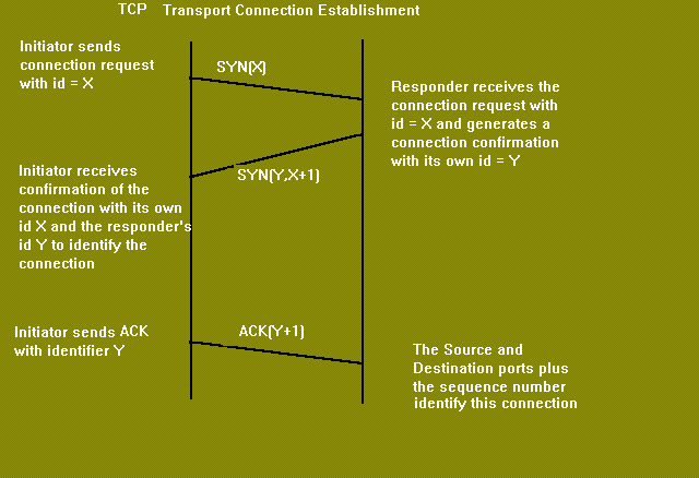
The "three-way handshake" is the procedure used to establish a connection. This procedure normally is initiated by one TCP and responded to by another TCP. The procedure also works if two TCP simultaneously initiate the procedure. When simultaneous attempt occurs, each TCP receives a "SYN" segment which carries no acknowledgment after it has sent a "SYN". Of course, the arrival of an old duplicate "SYN" segment can potentially make it appear, to the recipient, that a simultaneous connection initiation is in progress. Proper use of "reset" segments can disambiguate these cases.
The three-way handshake reduces the possibility of false connections. It is the implementation of a trade-off between memory and messages to provide information for this checking.
The simplest three-way handshake is shown in figure below. The figures should be interpreted in the following way. Each line is numbered for reference purposes. Right arrows (-->) indicate departure of a TCP segment from TCP A to TCP B, or arrival of a segment at B from A. Left arrows (<--), indicate the reverse. Ellipsis (...) indicates a segment which is still in the network (delayed). TCP states represent the state AFTER the departure or arrival of the segment (whose contents are shown in the center of each line). Segment contents are shown in abbreviated form, with sequence number, control flags, and ACK field. Other fields such as window, addresses, lengths, and text have been left out in the interest of clarity.

      TCP A                                                TCP B

  1.  CLOSED                                               LISTEN

  2.  SYN-SENT    --> <SEQ=100><CTL=SYN>               --> SYN-RECEIVED

  3.  ESTABLISHED <-- <SEQ=300><ACK=101><CTL=SYN,ACK>  <-- SYN-RECEIVED

  4.  ESTABLISHED --> <SEQ=101><ACK=301><CTL=ACK>       --> ESTABLISHED

  5.  ESTABLISHED --> <SEQ=101><ACK=301><CTL=ACK><DATA> --> ESTABLISHED

          Basic 3-Way Handshake for Connection Synchronisation
In line 2 of above figure, TCP A begins by sending a SYN segment indicating that it will use sequence numbers starting with sequence number 100. In line 3, TCP B sends a SYN and acknowledges the SYN it received from TCP A. Note that the acknowledgment field indicates TCP B is now expecting to hear sequence 101, acknowledging the SYN which occupied sequence 100.
At line 4, TCP A responds with an empty segment containing an ACK for TCP B's SYN; and in line 5, TCP A sends some data. Note that the sequence number of the segment in line 5 is the same as in line 4 because the ACK does not occupy sequence number space (if it did, we would wind up ACKing ACK's!).

Simultaneous initiation is only slightly more complex, as is shown in figure below. Each TCP cycles from CLOSED to SYN-SENT to SYN-RECEIVED to ESTABLISHED.

      TCP A                                            TCP B

  1.  CLOSED                                           CLOSED

  2.  SYN-SENT     --> <SEQ=100><CTL=SYN>              ...

  3.  SYN-RECEIVED <-- <SEQ=300><CTL=SYN>              <-- SYN-SENT

  4.               ... <SEQ=100><CTL=SYN>              --> SYN-RECEIVED

  5.  SYN-RECEIVED --> <SEQ=100><ACK=301><CTL=SYN,ACK> ...

  6.  ESTABLISHED  <-- <SEQ=300><ACK=101><CTL=SYN,ACK> <-- SYN-RECEIVED

  7.               ... <SEQ=101><ACK=301><CTL=ACK>     --> ESTABLISHED

                Simultaneous Connection Synchronisation
Question: Why is three-way handshake needed? What is the problem if we send only two packets and consider the connection established? What will be the problem from application's point of view? Will the packets be delivered to the wrong application?
Problem regarding 2-way handshake
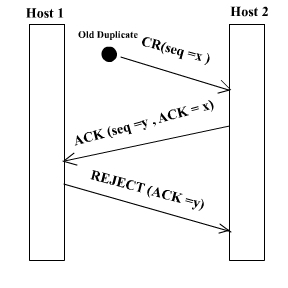
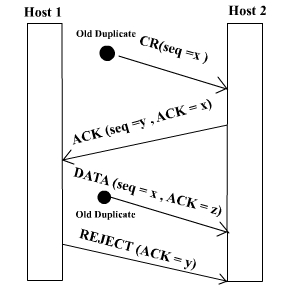
The only real problem with a 2-way handshake is that duplicate packets from a previous connection( which has been closed) between the two nodes might still be floating on the network. After a SYN has been sent to the responder, it might receive a duplicate packet of a previous connection and it would regard it as a packet from the current connection which would be undesirable.
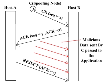
Again spoofing is another issue of concern if a two way handshake is used.Suppose there is a node C which sends connection request to B saying that it is A.Now B sends an ACK to A which it rejects & asks B to close connection.Beteween these two events C can send a lot of packets which will be delievered to the application..

The first two figures show how a three way handshake deals with problems of duplicate/delayed connection requests and duplicate/delayed connection acknowledgements in the network.The third figure highlights the problem of spoofing associated with a two way handshake. Some Conventions
1. The ACK contains 'x+1' if the sequence number received is 'x'.
2. If 'ISN' is the sequence number of the connection packet then 1st data packet has the seq number 'ISN+1'
3. Seq numbers are 32 bit.They are byte seq number(every byte has a seq number).With a packet 1st seq number and length of the packet is sent.
4. Acknowlegements are cummulative.
5. Acknowledgements have a seq number of their own but with a length 0.So the next data packet have the seq number same as ACK.

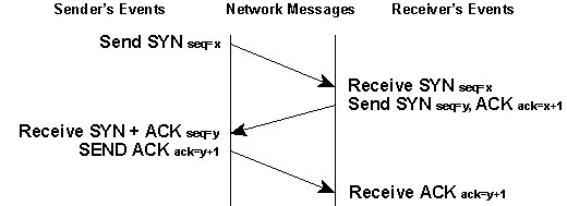
Connection Establish
  • The sender sends a SYN packet with serquence numvber say 'x'.
  • The receiver on receiving SYN packet responds with SYN packet with sequence number 'y' and ACK with seq number 'x+1'
  • On receiving both SYN and ACK packet, the sender responds with ACK packet with seq number 'y+1'
  • The receiver when receives ACK packet, initiates the connection.
Connection Release
  • The initiator sends a FIN with the current sequence and acknowledgement number.
  • The responder on receiving this informs the application program that it will receive no more data and sends an acknowledgement of the packet. The connection is now closed from one side.
  • Now the responder will follow similar steps to close the connection from its side. Once this is done the connection will be fully closed.


Transport Layer Protocol (continued)

TCP connection is a duplex connection. That means there is no difference between two sides once the connection is established.
Salient Features of TCP
  • Piggybacking of acknowledments:The ACK for the last received packet need not be sent as a new packet, but gets a free ride on the next outgoing data frame(using the ACK field in the frame header). The technique is temporarily delaying outgoing ACKs so that they can be hooked on the next outgoing data frame is known as piggybacking. But ACK can't be delayed for a long time if receiver(of the packet to be acknowledged) does not have any data to send.
  • Flow and congestion control:TCP takes care of flow control by ensuring that both ends have enough resources and both can handle the speed of data transfer of each other so that none of them gets overloaded with data. The term congestion control is used in almost the same context except that resources and speed of each router is also taken care of. The main concern is network resources in the latter case.
  • Multiplexing / Demultiplexing: Many application can be sending/receiving data at the same time. Data from all of them has to be multiplexed together. On receiving some data from lower layer, TCP has to decide which application is the recipient. This is called demultiplexing. TCP uses the concept of port number to do this.

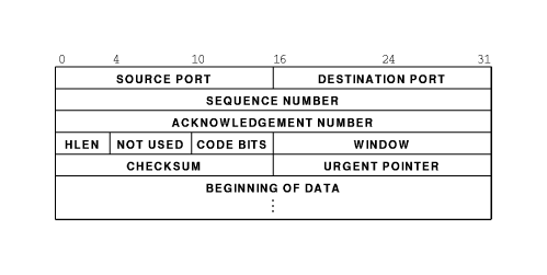
TCP segment header:

Explanation of header fields:
  • Source and destination port :These fields identify the local endpoint of the connection. Each host may decide for itself how to allocate its own ports starting at 1024. The source and destination socket numbers together identify the connection.
  • Sequence and ACK number : This field is used to give a sequence number to each and every byte transferred. This has an advantage over giving the sequence numbers to every packet because data of many small packets can be combined into one at the time of retransmission, if needed. The ACK signifies the next byte expected from the source and not the last byte received. The ACKs are cumulative instead of selective.Sequence number space is as large as 32-bit although 17 bits would have been enough if the packets were delivered in order. If packets reach in order, then according to the following formula:
    (sender's window size) + (receiver's window size) < (sequence number space)

    the sequence number space should be 17-bits. But packets may take different routes and reach out of order. So, we need a larger sequence number space. And for optimisation, this is 32-bits.
  • Header length :This field tells how many 32-bit words are contained in the TCP header. This is needed because the options field is of variable length.
  • Flags : There are six one-bit flags.
    1. URG : This bit indicates whether the urgent pointer field in this packet is being used.
    2. ACK :This bit is set to indicate the ACK number field in this packet is valid.
    3. PSH : This bit indicates PUSHed data. The receiver is requested to deliver the data to the application upon arrival and not buffer it until a full buffer has been received.
    4. RST : This flag is used to reset a connection that has become confused due to a host crash or some other reason.It is also used to reject an invalid segment or refuse an attempt to open a connection. This causes an abrupt end to the connection, if it existed.
    5. SYN : This bit is used to establish connections. The connection request(1st packet in 3-way handshake) has SYN=1 and ACK=0. The connection reply (2nd packet in 3-way handshake) has SYN=1 and ACK=1.
    6. FIN : This bit is used to release a connection. It specifies that the sender has no more fresh data to transmit. However, it will retransmit any lost or delayed packet. Also, it will continue to receive data from other side. Since SYN and FIN packets have to be acknowledged, they must have a sequence number even if they do not contain any data.
  • Window Size : Flow control in TCP is handled using a variable-size sliding window. The Window Size field tells how many bytes may be sent starting at the byte acknowledged. Sender can send the bytes with sequence number between (ACK#) to (ACK# + window size - 1) A window size of zero is legal and says that the bytes up to and including ACK# -1 have been received, but the receiver would like no more data for the moment. Permission to send can be granted later by sending a segment with the same ACK number and a nonzero Window Size field.
  • Checksum : This is provided for extreme reliability. It checksums the header, the data, and the conceptual pseudoheader. The pseudoheader contains the 32-bit IP address of the source and destination machines, the protocol number for TCP(6), and the byte count for the TCP segment (including the header).Including the pseudoheader in TCP checksum computation helps detect misdelivered packets, but doing so violates the protocol hierarchy since the IP addresses in it belong to the IP layer, not the TCP layer.
  • Urgent Pointer : Indicates a byte offset from the current sequence number at which urgent data are to be found. Urgent data continues till the end of the segment. This is not used in practice. The same effect can be had by using two TCP connections, one for transferring urgent data.
  • Options : Provides a way to add extra facilities not covered by the regular header. eg,
    • Maximum TCP payload that sender is willing to handle. The maximum size of segment is called MSS (Maximum Segment Size). At the time of handshake, both parties inform each other about their capacity. Minimum of the two is honoured. This information is sent in the options of the SYN packets of the three way handshake.
    • Window scale option can be used to increase the window size. It can be specified by telling the receiver that the window size should be interpreted by shifting it left by specified number of bits. This header option allows window size up to 230.
  • Data : This can be of variable size. TCP knows its size by looking at the IP size header.

Topics to be Discussed relating TCP

  1. Maximum Segment Size : It refers to the maximum size of segment ( MSS ) that is acceptable to both ends of the connection. TCP negotiates for MSS using OPTION field. In Internet environment MSS is to be selected optimally. An arbitrarily small segment size will result in poor bandwith utilization since Data to Overhead ratio remains low. On the other hand extremely large segment size will necessitate large IP Datagrams which require fragmentation. As there are finite chances of a fragment getting lost, segment size above "fragmentation threshold " decrease the Throughput. Theoretically an optimum segment size is the size that results in largest IP Datagram, which do not require fragmentation anywhere enroute from source to destination. However it is very difficult to find such an optimum segmet size. In system V a simple technique is used to identify MSS. If H1 and H2 are on the same network use MSS=1024. If on different networks then MSS=5000.
  2. Flow Control : TCP uses Sliding Window mechanism at octet level. The window size can be variable over time. This is achieved by utilizing the concept of "Window Advertisement" based on :
    1. Buffer availabilty at the receiver
    2. Network conditions ( traffic load etc.)
    In the former case receiver varies its window size depending upon the space available in its buffers. The window is referred as RECEIVE WINDOW (Recv_Win). When receiver buffer begin to fill it advertises a small Recv_Win so that the sender does'nt send more data than it can accept. If all buffers are full receiver sends a "Zero" size advertisement. It stops all transmission. When buffers become available receiver advertises a Non Zero widow to resume retransmission. The sender also periodically probes the "Zero" window to avoid any deadlock if the Non Zero Window advertisement from receiver is lost. The Variable size Recv_Win provides efficient end to end flow control.
    The second case arises when some intermediate node ( e.g. a router ) controls the source to reduce transmission rate. Here another window referred as COGESTION WINDOW (C_Win) is utilized. Advertisement of C_Win helps to check and avoid congestion.
  3. Congestion Control : Congestion is a condition of severe delay caused by an overload of datagrams at any intermediate node on the Internet. If unchecked it may feed on itself and finally the node may start dropping arriving datagrams.This can further aggravate congestion in the network resulting in congestion collapse. TCP uses two techniques to check congestion.
    1. Slow Start : At the time of start of a connection no information about network conditios is available. A Recv_Win size can be agreed upon however C_Win size is not known. Any arbitrary C_Win size can not be used because it may lead to congestion. TCP acts as if the window size is equal to the minimum of ( Recv_Win & C_Win). So following algorithm is used.
      1. Recv_Win=X
      2. SET C_Win=1
      3. for every ACK received C_Win++
    2. Multiplicative decrease : This scheme is used when congestion is encountered ( ie. when a segment is lost ). It works as follows. Reduce the congestion window by half if a segment is lost and exponentially backoff the timer ( double it ) for the segments within the reduced window. If the next segment also gets lost continue the above process. For successive losses this scheme reduces traffic into the connection exponentially thus allowing the intermediate nodes to clear their queues. Once congestion ends SLOW START is used to scale up the transmission.
  4. Congestion Avoidance : This procedure is used at the onset of congestion to minimize its effect on the network. When transmission is to be scaled up it should be done in such a way that it does'nt lead to congestion again. Following algorithm is used .
    1. At loss of a segment SET C_Win=1
    2. SET SLOW START THRESHOLD (SST) = Send_Win / 2
    3. Send segment
    4. If ACK Received, C_Win++ till C_Win <= SST
    5. else for each ACK C_Win += 1 / C_Win
  5. Time out and Retransmission : Following two schemes are used :
    1. Fast Retransmit
    2. Fast Recovery
    When a source sends a segment TCP sets a timer. If this value is set too low it will result in many unnecessary treransmissions. If set too high it results in wastage of banwidth and hence lower throughput. In Fast Retransmit scheme the timer value is set fairly higher than the RTT. The sender can therefore detect segment loss before the timer expires. This scheme presumes that the sender will get repeated ACK for a lost packet.
  6. Round Trip Time (RTT) : In Internet environment the segments may travel across different intermediate networks and through multiple routers. The networks and routers may have different delays, which may vary over time. The RTT therefore is also variable. It makes difficult to set timers. TCP allows varying timers by using an adaptive retransmission algorithm. It works as follows.
    1. Note the time (t1) when a segment is sent and the time (t2) when its ACK is received.
    2. Compute RTT(sample) = (t 2 - t 1 )
    3. Again Compute RTT(new) for next segment.
    4. Compute Average RTT by weighted average of old and new values of RTT
    5. RTT(est) = a *RTT(old) + (1-a) * RTT (new) where 0 < a < 1
      A high value of 'a' makes the estimated RTT insensitive to changes that last for a short time and RTT relies on the history of the network. A low value makes it sensitive to current state of the network. A typical value of 'a' is 0.75
    6. Compute Time Out = b * RTT(est) where b> 1
      A low value of 'b' will ensure quick detection of a packet loss. Any small delay will however cause unnecessary retransmission. A typical value of 'b' is kept at .2

Image References

  • http://plato.acadiau.ca/courses/comp/Eberbach/comp4343/lectures/transport/Com-TCP/f20_6.gif
if u like the post just say thank u in comment box.
Types, Construction, Working principle as an amplifier and characteristics of npn Teransistor


he NPN Transistor

In the previous tutorial we saw that the standard Bipolar Transistor or BJT, comes in two basic forms. An NPN (Negative-Positive-Negative) type and a PNP (Positive-Negative-Positive) type, with the most commonly used transistor type being the NPN Transistor. We also learnt that the junctions of the bipolar transistor can be biased in one of three different ways – Common Base, Common Emitter and Common Collector.
In this tutorial about bipolar transistors we will look more closely at the “Common Emitter” configuration using the Bipolar NPN Transistor with an example of the construction of a NPN transistor along with the transistors current flow characteristics is given below.

A Bipolar NPN Transistor Configuration

bipolar npn transistor configuration
(Note: Arrow defines the emitter and conventional current flow, “out” for a Bipolar NPN Transistor.)
 
The construction and terminal voltages for a Bipolar NPN Transistor are shown above. The voltage between the Base and Emitter ( VBE ), is positive at the Base and negative at the Emitter because for an NPN transistor, the Base terminal is always positive with respect to the Emitter. Also the Collector supply voltage is positive with respect to the Emitter ( VCE ). So for a bipolar NPN transistor to conduct the Collector is always more positive with respect to both the Base and the Emitter.
bipolar npn transistor NPN Transistor Connection
Then the voltage sources are connected to an NPN transistor as shown. The Collector is connected to the supply voltage VCC via the load resistor, RL which also acts to limit the maximum current flowing through the device. The Base supply voltage VB is connected to the Base resistor RB, which again is used to limit the maximum Base current.
We know that the transistor is a “current” operated device (Beta model) and that a large current ( Ic ) flows freely through the device between the collector and the emitter terminals when the transistor is switched “fully-ON”. However, this only happens when a small biasing current ( Ib ) is flowing into the base terminal of the transistor at the same time thus allowing the Base to act as a sort of current control input.
The transistor current in a bipolar NPN transistor is the ratio of these two currents ( Ic/Ib ), called the DC Current Gain of the device and is given the symbol of hfe or nowadays Beta, ( β ). The value of β can be large up to 200 for standard transistors, and it is this large ratio between Ic and Ib that makes the bipolar NPN transistor a useful amplifying device when used in its active region as Ib provides the input and Ic provides the output. Note that Beta has no units as it is a ratio.
Also, the current gain of the transistor from the Collector terminal to the Emitter terminal, Ic/Ie, is called Alpha, ( α ), and is a function of the transistor itself (electrons diffusing across the junction). As the emitter current Ie is the sum of a very small base current plus a very large collector current, the value of alpha α, is very close to unity, and for a typical low-power signal transistor this value ranges from about 0.950 to 0.999

α and β Relationship in a NPN Transistor

npn transistor alpha beta relationship
 
By combining the two parameters α and β we can produce two mathematical expressions that gives the relationship between the different currents flowing in the transistor.
transistor alpha and beta relationship
 
The values of Beta vary from about 20 for high current power transistors to well over 1000 for high frequency low power type bipolar transistors. The value of Beta for most standard NPN transistors can be found in the manufactures data sheets but generally range between 50 – 200.
The equation above for Beta can also be re-arranged to make Ic as the subject, and with a zero base current ( Ib = 0 ) the resultant collector current Ic will also be zero, ( β x 0 ). Also when the base current is high the corresponding collector current will also be high resulting in the base current controlling the collector current. One of the most important properties of the Bipolar Junction Transistor is that a small base current can control a much larger collector current. Consider the following example.

NPN Transistor Example No1

A bipolar NPN transistor has a DC current gain, (Beta) value of 200. Calculate the base current Ib required to switch a resistive load of 4mA.
npn transistor base current
 
Therefore, β = 200, Ic = 4mA and Ib = 20µA.
One other point to remember about Bipolar NPN Transistors. The collector voltage, ( Vc ) must be greater and positive with respect to the emitter voltage, ( Ve ) to allow current to flow through the transistor between the collector-emitter junctions. Also, there is a voltage drop between the Base and the Emitter terminal of about 0.7v (one diode volt drop) for silicon devices as the input characteristics of an NPN Transistor are of a forward biased diode.
Then the base voltage, ( Vbe ) of a NPN transistor must be greater than this 0.7V otherwise the transistor will not conduct with the base current given as.
npn transistor base current formula
 
Where:   Ib is the base current, Vb is the base bias voltage, Vbe is the base-emitter volt drop (0.7v) and Rb is the base input resistor. Increasing Ib, Vbe slowly increases to 0.7V but Ic rises exponentially.

NPN Transistor Example No2

An NPN Transistor has a DC base bias voltage, Vb of 10v and an input base resistor, Rb of 100kΩ. What will be the value of the base current into the transistor.
base current calculation
 
Therefore, Ib = 93µA.

The Common Emitter Configuration.

As well as being used as a semiconductor switch to turn load currents “ON” or “OFF” by controlling the Base signal to the transistor in ether its saturation or cut-off regions, Bipolar NPN Transistors can also be used in its active region to produce a circuit which will amplify any small AC signal applied to its Base terminal with the Emitter grounded.
If a suitable DC “biasing” voltage is firstly applied to the transistors Base terminal thus allowing it to always operate within its linear active region, an inverting amplifier circuit called a single stage common emitter amplifier is produced.
One such Common Emitter Amplifier configuration of an NPN transistor is called a Class A Amplifier. A “Class A Amplifier” operation is one where the transistors Base terminal is biased in such a way as to forward bias the Base-emitter junction.
The result is that the transistor is always operating halfway between its cut-off and saturation regions, thereby allowing the transistor amplifier to accurately reproduce the positive and negative halves of any AC input signal superimposed upon this DC biasing voltage.
Without this “Bias Voltage” only one half of the input waveform would be amplified. This common emitter amplifier configuration using an NPN transistor has many applications but is commonly used in audio circuits such as pre-amplifier and power amplifier stages.
With reference to the Common Emitter Configuration shown below, a family of curves known as the Output Characteristics Curves, relates the output collector current, ( Ic ) to the collector voltage, ( Vce ) when different values of Base current, ( Ib ). Output characteristics curves are applied to the transistor for transistors with the same β value.
A DC “Load Line” can also be drawn onto the output characteristics curves to show all the possible operating points when different values of base current are applied. It is necessary to set the initial value of Vce correctly to allow the output voltage to vary both up and down when amplifying AC input signals and this is called setting the operating point or Quiescent Point, Q-point for short and this is shown below.

Single Stage Common Emitter Amplifier Circuit

common emitter amplifier
 

Output Characteristics Curves of a Typical Bipolar Transistor

transistor collector characteristics
 
The most important factor to notice is the effect of Vce upon the collector current Ic when Vce is greater than about 1.0 volts. We can see that Ic is largely unaffected by changes in Vce above this value and instead it is almost entirely controlled by the base current, Ib. When this happens we can say then that the output circuit represents that of a “Constant Current Source”.
It can also be seen from the common emitter circuit above that the emitter current Ie is the sum of the collector current, Ic and the base current, Ib, added together so we can also say that Ie = Ic + Ib for the common emitter (CE) configuration.
By using the output characteristics curves in our example above and also Ohm´s Law, the current flowing through the load resistor, ( RL ), is equal to the collector current, Ic entering the transistor which in turn corresponds to the supply voltage, ( Vcc ) minus the voltage drop between the collector and the emitter terminals, ( Vce ) and is given as:
npn transistor collector current
 
Also, a straight line representing the Dynamic Load Line of the transistor can be drawn directly onto the graph of curves above from the point of “Saturation” ( A ) when Vce = 0 to the point of “Cut-off” ( B ) when Ic = 0 thus giving us the “Operating” or Q-point of the transistor. These two points are joined together by a straight line and any position along this straight line represents the “Active Region” of the transistor. The actual position of the load line on the characteristics curves can be calculated as follows:
npn transistor load line
 
Then, the collector or output characteristics curves for Common Emitter NPN Transistors can be used to predict the Collector current, Ic, when given Vce and the Base current, Ib. A Load Line can also be constructed onto the curves to determine a suitable Operating or Q-point which can be set by adjustment of the base current. The slope of this load line is equal to the reciprocal of the load resistance which is given as: -1/RL
Then we can define a NPN Transistor as being normally “OFF” but a small input current and a small positive voltage at its Base ( B ) relative to its Emitter ( E ) will turn it “ON” allowing a much large Collector-Emitter current to flow. NPN transistors conduct when Vc is much greater than Ve.
In the next tutorial about Bipolar Transistors, we will look at the opposite or complementary form of the NPN Transistor called the PNP Transistor and show that the PNP Transistor has very similar characteristics to the bipolar NPN transistor except that the polarities (or biasing) of the current and voltage directions are reversed.